Occultation campaign example

On 2025 August 19, an occultation occurred, visible across a broad swath of the United States. This article delves into the why, who, what and where of this campaign.

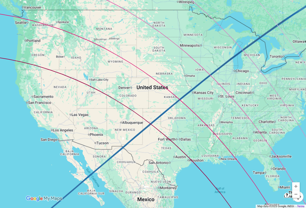
The blue line shows the predicted shadow path. At this scale, you can’t see the size of the asteroid, but you get a rough idea of where to go to see the occultation. The arced lines show where the object is 30° above the horizon, and then 5° lower for each successive arc moving to the northeast. From Baja, Mexico, the star is highest in the sky. Moving to the northeast along the line, the asteroid gets closer and closer to the horizon. The areas we were looking at stretched from the western tip of Texas up through Kansas.

The asteroid in this case is (59980) 1999SG6. This is an otherwise unremarkable asteroid, soon to meet a date with destiny that makes chasing this one down more interesting. There is a mission under development in the United Arab Emirates called the Emirati Mission to the Asteroids (EMA). Scheduled for launch in 2028, the spacecraft will fly by six asteroids and then go into orbit around a seventh asteroid, (629) Justitia.

The launch date plus the goal of orbiting Justitia provides an opportunity to visit other asteroids along the way, and the six extra bodies are the ones close enough to be interesting. That circumstance seems rather amazing, flying in the asteroid belt for 7 years and there are only six other asteroids you can get close to. It’s even more amazing given that this spacecraft has active propulsion throughout the mission and will be constantly changing its orbit to meet its date with each target. Space really is mostly empty.

The Asteroid

What do we know, or conversely, what do we not know about (59980) 1999SG6? As you can see, we don’t even know its name yet. This descriptor is fine for computers, but it is rather cumbersome to use here. I will use the abbreviation common to see these days, SG6, to refer to the asteroid. Someday soon I hope we’ll have something better.

SG6 was officially discovered in 1999, but observations have been recovered that go back for 40 years. Its orbit has a semi-major axis of 3.05 AU (Earth is at 1 AU), is nearly circular with an eccentricity of 0.03, and is inclined by 11° from the plane of the solar system. Estimates of its size indicate that it is 8 km across and that it rotates once every 2.27 hours. The reflectivity of its surface is about 12%, similar to the Moon.

So far, there isn’t much information on the shape of SG6. Two previous occultations were attempted. The first was foiled by weather, and the second provided a good position for the asteroid but confusing details about the shape. We’re still working on those results but had to press on to the next opportunity with our best guesses.

The Opportunity

There are a lot of occultations by SG6. In the next 10 years, I found more than 530 events scattered all over the Earth. One event on the list was on 2025 August 19. What made this event so special was its location. The predicted shadow path crossed over Wichita, Kansas, on a line that extended down to El Paso, Texas. Most of the region is an 8 hour drive from the Boulder, Colorado area.

A group of students from the University of Virginia contacted me to see if I was interested. Thanks to the previous occultation that they did near Georgia, the prediction was updated and was to be very precisely located. The path of the asteroid shadow had a 68% chance of falling within ±1.2 km of the prediction. With this low uncertainty, it becomes possible to deploy many stations across the shadow to produce a very detailed shape.

The star was faint enough that larger telescopes were required. My systems are mostly 28-cm telescopes that were just barely big enough. I was working to provide training for a student from the University of Sharjah. The coincidence in the dates of that training trip and the occultation provided a perfect opportunity for the trainee to witness the development and execution of an occultation campaign.

The Campaign Design

Every campaign should start with a goal. My preference is to pursue a scientifically useful result from the large group effort. In this case, our primary goal is to obtain a detailed shape for SG6. If successful, we would also learn the absolute size and thus the albedo of the surface. The low uncertainty gave us some confidence in achieving the goals.

There are four key parameters that define a campaign, but only two of these are generally under our control. These parameters are:

1. Size and shape of the object.

2. Uncertainty of the position of the shadow track.

3. The chance of success.

4. The spatial resolution of the shape.

The first item is clearly out of our control, and all we can do is work off our best guess and a possible (or probably) range that is allowed. Previous research predicts a circular-equivalent diameter of 8 km. No one knows if the object is circular, elliptical, or any of the other complex possibilities seen with small asteroids. For this event, I considered the size to be more uncertain than the location of the shadow.

The second item clearly tells you where to go to see the occultation. If this is wrong, you won’t see anything interesting. Not too long ago, this was the entire story and controlled every aspect of doing occultation science. With data from the Gaia mission, we know where the stars are. We are also getting better and better information about where the asteroids are since we measure their positions against the Gaia catalog star coordinates. In the past 10 years, the quality of the orbits for main-belt asteroids has improved dramatically. Then, when you can add a prior occultation result or two, the prediction can be extremely precise. That is the case for this opportunity. In the end, yes, you can actively work to reduce the uncertainties, but it’s not something you can do quickly. Astrometry from traditional means or occultations takes years to build up to a useful level. When you are in the last couple of weeks before an event, the prediction you have is what you have to deal with.

Now we get to the components of the problem that we get to design. The number of telescope stations available connects the chance for success and the spatial resolution goal. If you know two of these things, you can calculate the third.

I have a tool that lets me simulate an occultation with one or more stations. The resulting calculation tells me the probability that a station will see the event. By adding up a set of stations, I can then determine the probability of success for the entire campaign.

For a single station, the probability depends on three things: the size of the object, the uncertainty of the prediction, and the distance of the station from the predicted center of the shadow. The highest probability is always at the center of the shadow and decreases as the distance increases. There are a lot of fun details in this problem, but I’m going to leave that for another day. A qualitative understanding is sufficient for now. Clearly, if the object is large and the orbit uncertainty is small compared to the size, being closer to the centerline than the radius of the object will ensure success for a station. With this event, the ratio of the radius to the uncertainty is 4/1.2 or 3.3. That is a good number, but not big enough to let us ignore the uncertainties. However, when this ratio is greater than one, going after a detailed shape is a practical goal.

The practical side of a spatial resolution goal emerges when you figure out the number of telescopes you need. If there is no uncertainty, the calculation is simple. If the object is 8 km across and you want 500 m sampling of the profile, you need 17 stations (diameter/spacing+1). In this case, all stations see something, though the ones on the very edge might see a blip that is too short to measure. In my tools, I assume that any station located further than 80% of the radius from the center won’t see an event because it is too short. This isn’t always true, but my approach provides a conservative estimate of the outcome of the campaign.

Let’s put this all together with some simple math. Let N be the number of stations to deploy. Let σ represent the uncertainty in the centerline's position (aka, center of the shadow). Next, let Δ be the spacing between stations. Finally, let’s use s to scale the size of the probability zone to cover. We already have D for the diameter. To find the number of stations, use N = (2sσ+D)/Δ+1. The quantity, 2sσ+D, is what I call the spread. This is the distance from one end of the coverage to the other and tells you something right away about how much driving might be involved.

For this campaign, I chose s=3. This is also known as a 3σ plan and means that 98% of the probability space for the event is covered. I have run campaigns with s as low as 0 and as high as 5. This is always a difficult and subjective decision. I strive to strike a balance between the effort and cost of an event and the odds for success. Whatever the decision might be, I always know what value of s will be used for the event.

The next trade-off in the campaign design is settling on the number of stations and the spacing. Here are some examples. If Δ=0.5 km, our 3σ plan would have a spread of 15.2 km, requiring 31.4 (rounded to 31) stations. This campaign design would provide an excellent result but was too large for an unfunded effort. I have plenty of equipment and people to do the work, but the lack of funding restricts the pool of observers to a handful of the most enthusiastic.

Our final tally of observers came to 11. Two observers were working as a team so if each observer-team used one telescope, the number of stations would be 10. Keeping the spread the same leaves us with a spacing of 1.7 km where we could expect to get 3-4 positive detections from the 10 stations.

These two cases provided the bounds for the plan. Fewer than 10 stations felt like it wasn’t worth the effort, but a goal of 31 stations was out of reach. The team decided on a more difficult strategy of some teams deploying more than one station. One observer signed up to do three stations and six observers felt comfortable running two stations. That decision brought the station total up to 18 and a spacing of 1.2 km between stations.

One important aspect here is not entirely obvious. Defining campaigns in this way naturally leads to a regular pattern of coverage across the object. This regularity provides the most information for a given number of stations. If the pattern is random, there will be larger gaps and smaller gaps, both of which reduce the amount of information.

The goal of a regular deployment pattern has important considerations: how best to incorporate fixed sites, how to address weather uncertainties, and what to do when observers cancel or new observers appear at the last minute.

Fixed sites are challenging since they cannot be moved to be in the optimum location. Do we drop the nearest “perfect” track or pretend that the fixed site doesn’t exist? With this campaign, I shifted the overall pattern by 70 meters to put one of the regularly spaced tracks on top of the one fixed observatory. That shift wasn’t big enough to change the outcome and was a suitable compromise.

The last consideration is far more serious. Before the pattern of stations is set, we can adjust the spacing between by a small amount and maintain the regular pattern. This works equally well for additions and cancellations. Once the station count is set, the pattern can be defined, enabling the teams to begin site scouting and planning. There is a tension between adapting to the changing size of the team and providing ample time for site planning. Reducing the number of stations within the last 48 hours is always very damaging to the deployment plan. Adding stations isn’t as bad, but it means that the amount of information added by extra stations is far less than it could be. Chasing an occultation requires effort, and I always want to get the most for the effort that I can.

After all of this planning, the final deployment plan emerged. The image shown below zooms in on the deployment region near Wichita, Kansas. There are five dark diagonal lines. The center of these is the predicted path of the center of the asteroid. The next pair of lines outward from the center is the expected size of the object, 8 km from edge to edge. Finally, the outermost pair of dark lines shows the 3σ orbit uncertainty limit. The magenta lines show the deployment plan with lines of constant distance from the center.

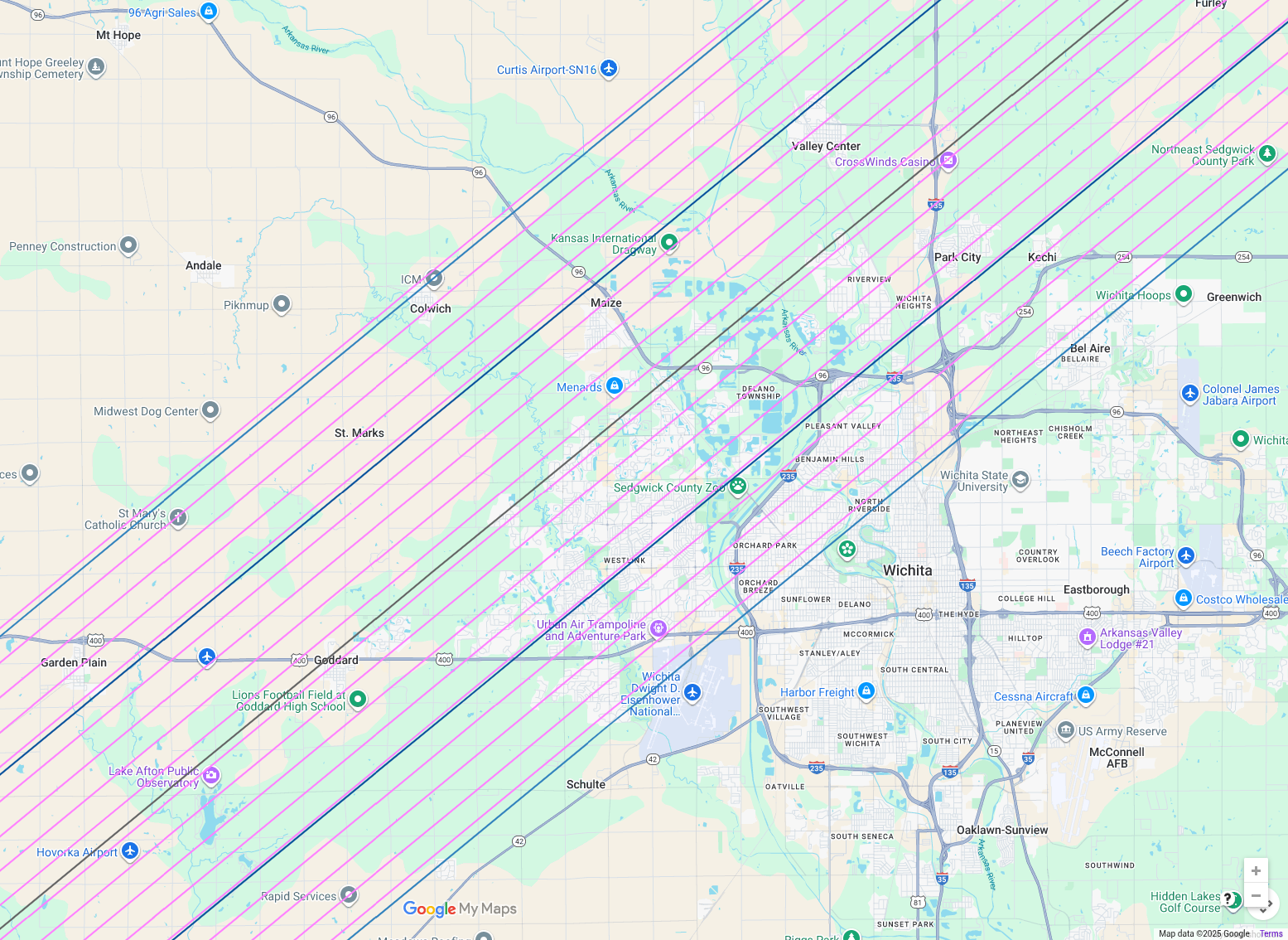
The magenta lines are provided as high-resolution kml files suitable for loading in a map application on a cell phone. Each observer is assigned their tracks and their job becomes finding a place to observe that is on their track. For this event, I asked that everyone be within 45 meters of their line. Any location on a single track is as good as any other. This factor of mobility along the track is the only thing that we can use to escape bad weather.

The Deployment

Weather uncertainties can mean a localized area could be systematically wiped out if a group of stations are all in a similar area. For this event, some teams wanted to work to the northeast of Wichita, and other teams preferred the southwest area. The chances of clear or cloudy skies seemed to be similar but far enough apart that one or the other, but not both, could be good or bad. Under such circumstances, I try to interleave the two groups so that a dropout from one group just reduces the density of the chords in the shadow rather than creating a much larger gap in the coverage. When built into the plan from the start, this can be very effective. This time, the decision to split up was made just hours before the event, and the distribution of locations was not as resilient as it could have been. But, as I say to all my teams, it’s impossible to optimize the outcome when fighting the weather. Our best efforts will have to suffice.

Similar to weather-induced failures, it is also possible for the observers to make mistakes or have problems that remove them from the experiment. Since we were trying to deploy multiple stations by a single observer, a problem could lead to losing both stations, leaving a much larger gap in the coverage. The assignment of locations did not assign the same observer to adjacent tracks. This made things slightly harder on the observers, but the spacing between sites was so small it ended up being a minor factor.

In the week leading up to the campaign, one factor remained. The weather forecast was not good. Even worse, the forecast kept changing. I tracked the weather in Wichita, Amarillo, Roswell, and Las Cruces to maintain a larger picture of where we would find the best weather.

The driving requirements led to the decision to meet the night before the event in the Wichita area, and we ended up in Goddard, Kansas. The plan was to evaluate the weather on the morning of the event. If needed, we could have driven as far as Roswell. The forecast in Roswell was particularly troublesome. Sometimes it was predicted to be cloudy and rainy, and then the next prediction said it was going to be clear.

In the end, it seemed like there was no clear winner. All our choices were similarly uncertain. We made the choice to stick closer to Wichita. Instead of investing in a long drive with no clear chance of improving the weather odds, we used the time to better scout the nearby region for places to set up. This advance work can really help minimize effort and risk for getting set up in time at the right place.

Below is a satellite image taken near‌ the time of the occultation. The best region was clearly in southeastern Kansas, but if you look closely, you can see faint tendrils of cloud in the area we needed to be in.

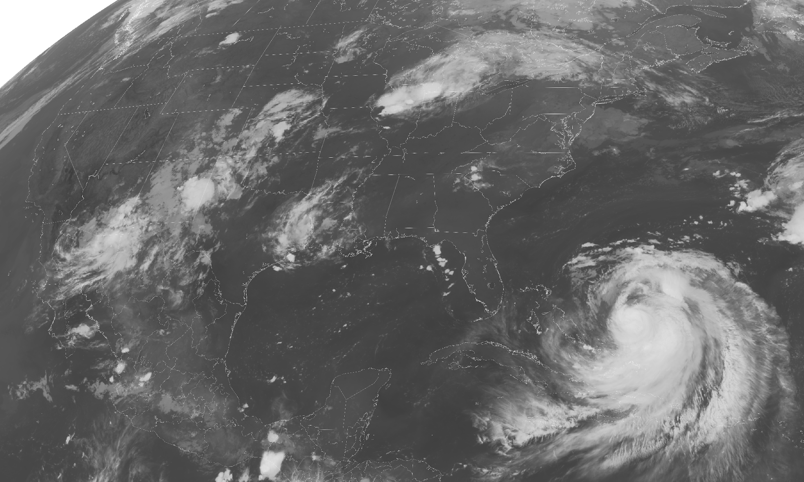
Every team struggled with a last-minute decision on where to go. In the final 12 hours before the event, we stopped looking at forecasts. Instead, we relied on satellite images like the picture above plus what we could see looking out the window. In the end, we did pretty well. Though six sites were foiled by weather, twelve collected useful data. The strategy of mixing up teams and tracks worked really well. There were no adjacent site failures.

I won’t go into all the details about how we evaluated and tracked the weather. There were a lot of discussions, and everyone had their own take on what we were seeing. However, the collective focus was on avoiding clouds. That seems like an obvious thing to do, and we weren’t wrong. I suspect one reason the weather was acting so strange is the influence of Hurricane Erin, which you can see here east of Florida. These storms can mess with the weather pattern of an area much larger than the hurricane itself. I’m sure it was an influence along the shadow path, making it much harder to predict than normal.

There was one factor that we didn’t consider, and that became my personal lesson learned from this effort. Humidity. I thought everyone was close enough together that the water vapor in the air would be the same everywhere. Maybe it was. But if you are close to the dew point, just a little more or less water, or, a slightly lower temperature (even just 0.5 degrees) can mean one area will be prone to form dew on the telescope optics before the other. Everyone who went to the northeast of Wichita struggled with dew, and this was the dominant reason for those site failures. Sites to the southwest didn’t have that problem. We held our own against the clouds, but the humidity snuck up on us. I’m not even sure I know how to avoid this in the future. It’s not at all clear that dew shields or dew heaters would have helped. Perhaps it’s impossible to get the appropriate high-resolution and fidelity information to predict the dew point well enough to matter.

The Result

Four of the sites with good data recorded a positive occultation. The rest are all negative constraints, and there were negatives on both sides of the clump of positives. Having bounding negatives is extremely important. Those data establish a very strong upper limit to the size. In this case, we now know the cross-track size of the object cannot be larger than 6.2 km or smaller than 3.7 km. Also, we know the object has a circular profile. It must be elliptical or some other irregular shape. The down-track axis of the body appears to be around 6 km. This size is quite surprising. Remember that our best guess was an 8 km diameter. Our results show that the object we saw is 35 to 58% smaller in projected area than predicted.

The precise shape remains elusive. Our data were very noisy due to either clouds or dew on the optics. The timing uncertainties of the edge points are similar in size to the topography on the object. We will need to try this object again, but the next campaign will benefit from this effort and be more effective for what we’ve learned. By all measures, this was a successful campaign. The weather did its best to shut us down, but the group effort prevailed in the end. Kudos to the team: Kai, Anoud, Vadim, Gary, Brian, Chet, Keya, Andrey, Teddy, Uday, and Roger. This was a heroic effort. Congratulations, one and all, on a job well done. Now we just have to sit down and write up the results for a scientific publication. At the beginning, I said this was an unremarkable asteroid. I’ve lost track of how many times I’ve said that and then find that it’s interesting after all. I think this asteroid is turning out to be interesting after all. Perhaps I should just say that all asteroids are interesting. I really don’t have a problem with that.