Observing strategy: exposure time
How fast (or slow) should I go?

One important feature of the occultation predictions I provide is some guidance on the rate of data collection. In this article, I want to describe my approach to picking a recommended exposure time. But first, let’s cover some background information.
For video systems, we usually refer to the frame rate, or the number of images collected per second. With NTSC video (common in the US), the rate is 29.97 frames/second. This number is the reciprocal of the exposure time. Thus, the exposure time for NTSC video is 0.033 seconds (rounded to the nearest milli-second). The video standard fixes this rate, but there are tricks played by some cameras that can decrease the frame rate by integer values, though powers of two are most often used.
With the old RECON systems, our video cameras had a setting called SENSEUP that was the frame-rate integration factor. Actually, this factor is the field-rate integration factor because NSTC video is made up of fields, two per frame. This means that full-speed video and a SENSEUP of 2x have the same frame rate. A SENSEUP of 4x has an exposure time two times longer at 0.067 seconds. The longest exposure time was for a SENSEUP of 128x, equivalent to 2.1 seconds.
The newer camera we use in the RECON project and elsewhere is the QHY174M-GPS. This is a digital imaging camera based on a CMOS detector similar to what you have built into your cell phone. This system has a built-in GPS receiver that is used to implant data in each image to record the location (latitude, longitude, and altitude) and the time for each image. Another important feature of CMOS cameras is the short time needed to read and save the image, less than a thousandth of a second for the QHY174.
Unlike a video camera, we have complete control over the duration of an exposure with a CMOS camera. I have used exposure times over a range from 0.000002 seconds up to 30 seconds. This isn’t the full range of what the camera can do, but that is already more than we need for occultations.
Choosing an exposure time means balancing the image collection rate and the quality of the observation. Let’s break this down.
At first glance, you might assume that faster is always better. This assumption is correct up to a point. Clearly, if you go too slow, you won’t see anything. Using an exposure time of 30 seconds for an occultation that lasts a fraction of a second isn’t likely to tell you very much.
The occultations we observe involve a very distant light source and an obscuring body that is not as far away. To a very good approximation, this situation matches that of diffraction from a knife edge. Augustin-Jean Fresnel worked out the physics of light diffraction that applies here and I encourage you to read more if you want to know the details.
Without diffraction, the signal from a star would disappear instantly, assuming the star has no angular size. In this case, the faster you go, the more accurate you can time the instant the star disappears and reappears. Diffraction, and to a lesser extent a finite star size, blurs out the brightness of the star as a function of time during an occultation. If the occulting body is small enough, the diffraction patterns from both sides of the object interact, further complicating what you see.
Fresnel diffraction hides details finer than 2 km for a distance twice as far as Neptune and Pluto. I would set the lower bound for the exposure time to be something that gives 1 km spacing between points. You gain nothing by going faster. For a typical shadow speed of 20 km/sec, the shortest useful exposure time is 0.05 seconds. Main-belt asteroids are closer and their limit is smaller at roughly 200 meters. In this case, the shortest exposure time would be 0.01 seconds. My descriptions here are necessarily incomplete. I’m focused primarily on small, but not too small asteroids. If you want a broader perspective, take a looks at a recent review article that digs into a lot more details.
The actual limit clearly varies depending on the event and the distance to the target. For most occultations, diffraction does not matter. Other factors are more important.
This discussion now needs to turn to noise. We want to measure the signal from the star over a finite exposure time, but what we really need to know is how good that measurement will be. The technical term for this the signal-to-noise ratio, commonly abbreviated as SNR. High SNR data is better than low SNR data. As the exposure time increases, the SNR also increases. A rough rule-of-thumb is that increasing the exposure time by a factor of four will increase the SNR by a factor of two. Ah, if it were just that easy…
I will not go into all the details here, but I have a theoretical model, initially created by Mike Skrutskie from the University of Virginia. I adapted this model for automated use by the RECON project and included some testing and verification.
The model includes some basic parameterization of the equipment and our observing environment here on Earth. We need the size of the telescope, of course. But, we also need to know its focal length, the size of typical images, and how that maps onto the pixels in the camera. These factors define the expected signal.
The noise is a lot more complicated and harder to predict. The expected sky brightness is important, as is the readout noise in the camera. Scintillation is another more complicated noise source, most commonly known as how the stars “twinkle” at night. This factor is increasingly important as the telescope aperture size decreases. Any signal that is detected is subject to “photon-counting” noise. This applies equally to photons from the star, from the asteroid, and from the sky.
Given these factors, there are three variables to be set for an occultation: star brightness, asteroid brightness, and shadow speed. These will determine the SNR as a function of exposure time. Knowing the expected size of the asteroid sets the range of useful exposure times.
All of what I explained is useful, but when it comes time to observe, we really just want to know the exposure time. Below is the algorithm behind my determinations. Note that the answer depends on the system to be used and I have chosen the RECON standard system for my predictions and for this example: a CPC1100 telescope, QHY174 camera, and a 2x focal reducer with a diagonal.
Setup: The exposure time must fall between 0.12 and 2 seconds. Create a vector of exposure times at 0.01 second intervals between 0.12 and 0.25 seconds and then at 0.05 second intervals between 0.25 and 2.0 seconds. Compute the SNR for all candidate exposure times. Compute the number of samples across a diameter for each exposure time option.
Find all cases with 5 ≤ SNR ≤ 10 and 4 or more samples. If there is more than one choice, keep the highest SNR option as the chosen exposure time. If no choices meet these criteria, go on to the next step. This is Zone 1 in the plot.
Find all choices with SNR ≥ 5 and with 4 or more samples. If there is more than one choice, keep the lowest SNR option as the chosen exposure time. If no choices meet these criteria, go on to the next step. This is Zone 2 in the plot.
Find all choices with SNR ≥ 3 and with 4 or more samples. If there is more than one choice, use the exposure time for the highest SNR case. If no choices meet these criteria, go on to the next step. This is Zone 3 in the plot.
Find all choices with SNR ≥ 3 and with 2 or more samples. If there is more than one choice, keep the exposure time with the highest SNR case. If no choices meet these criteria, the event is not worth observing. This is Zone 4 in the plot.
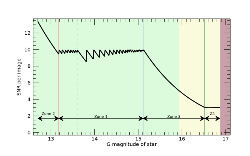
Figure 1 illustrates the behavior of the program. The star brightness is highest on the left, lowest on the right of the plot. The green zones shows cases where good data are ensured, with SNR ≥ 5. Anything in this zone will provide excellent data under clear skies. The yellow zone is not really where we want to be but the data will be usable, if not a little difficult to process. The red zone is beyond the capability of this system and is a waste of time.
Here is the underlying logic. Zone 1 is in the “sweet spot” of sampling and SNR. There are many choices that will return good data. My choice here is to not get greedy, go slower and take the highest SNR. The sawtooth pattern in the curve is a consequence of the discretized exposure time. Zone 2 includes cases where the star is very bright and gives good data at even the fastest exposure time. There really aren’t any adjustments that can be made here. However, using shortest valid exposure time provides excellent spatial resolution to search for rings and small satellites. Zone 3 covers cases at lower SNR than we’d really like. Here, I insist on at least 4 images across the diameter while maintaining a useful SNR. Zone 4 is the last ditch option. Relax the sampling to just two points across the diameter with SNR≥3.
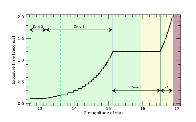
This scheme is not what I started with when originally writing the software. The deciding factor in the choice of logic was an additional constraint to ensure that, as the target star brightness increases (for sample cases), the exposure time never decreases. The plot below shows the exposure time for each case plotted in the first figure. Note how the curve is flat or descends as you move from right to left. This factor is responsible for Step 1 being a little different from the rest. The dashed green vertical line is the transition from 0.01 to 0.05 second steps in the exposure time.
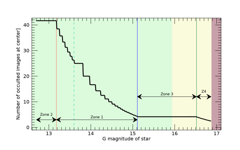
The number of occulted images on the centerline provides view of the last portion of the logic used. The figure below shows how the number of samples decreases as the star brightness decreases. You can see how how the requirement of 4 samples across the object freezes the exposure time the SNR drops with decreasing stellar brightness. Eventually, you run out of room and the last zone is dictated by the SNR being clamped at 3 and the number of samples steadily decreases. As soon as you get to a brightness that cannot give you SNR=3 and 2 samples, those fainter stars are of no use.
There is one more subtle condition to be aware of. The brightness of the asteroid is not fully considered in all these steps. The computed SNR is for the unocculted signal. During an occultation you only see light reflecting from the asteroid. If the asteroid is bright enough, it becomes hard to tell if the star disappears.
My model does include the effect of the asteroid and I provide an SNR value for the drop in brightness in addition to the unocculted SNR but does not affect the exposure time calculation. Why not use the flux drop SNR to set the exposure time? The problem is that the predicted brightness of the asteroid can be very wrong. I prefer to leave this point up to the observer to decide. Just last week, I observed an occultation where the asteroid was predicted to be 2-3x brighter than the star. If this was correct, an occultation would be impossible to detect without a very large telescope. But, when I got on the field an hour before the event, I could clearly see both the star and asteroid. Yes, the asteroid was brighter, but only by a small amount. In the end, the prediction was pessimistic, and we got a detection after all. Sometimes you just have to take a chance.
What should you do if you don’t have a standard RECON system? In this case, you need to figure out a scaling factor from my system to yours. The biggest factor is the aperture of your telescope and a simple scaling on this basis is often good enough. Let’s say you have an 8-inch telescope. The ratio of the areas of the primary mirrors is (8/11)2 and implies that you get 85% less light in the same amount of time. If you collect the same amount of light, you would get nearly the same SNR. So, if the exposure time is give as 1 second for an 11”, you would want to use 1.17 seconds on an 8” to compensate for the smaller mirror. This adjustment is fine as long as the event falls in Zones 1 and 2. If the event is in the other two zones, you need to check to make sure that the slower cadence isn’t going to be a problem for that event. The is no getting around the fact that a smaller telescope can’t work on stars as faint as those visible in larger telescopes.
Another factor in adjusting for your system is the total throughput of the two systems. There is no telescope and camera that can measure 100% of the light that hits the system. Every lens, mirror, and window in the system will cause some light to be lost and the detector itself is not perfectly efficient. Most systems fall some where between 40-80% throughput. Generally speaking, most systems are all about the same efficiency and I usually ignore this factor. However, if you consistently find that you get better or worse data than my SNR prediction and your aperture correction indicates, it may just be that the throughput is different. With data and experience, you can figure out your own correction factor.
There are some caveats to my approach. It is not possible to predict everything related to the SNR. Sky brightness is one confounding factor. Light pollution does matter but so does the moon. In fact, the moon is a bigger factor for all but the largest urban areas. The phase of the moon, angular distance of the occultation star from the moon, dust in the atmosphere, and clouds (thin or otherwise), all contribute to the sky background. My tool attempts a value for middling conditions, not super great but also not super bad.
The image quality, or seeing, also affects the data quality and SNR. You can’t do much about bad seeing from the atmosphere but focus is something you need to take very seriously since that is under your control. In any case, my calculations assume image quality of about 2.5 arcsec, not fantastic but not bad.
Knowing that a perfect prediction isn’t possible, I build into my system a little bit of margin. That means a problem, known or unknown, that crops up and reduces the SNR won’t be instantly fatal to the observation. There was a time when I recommended making on-site adjustments to the requested exposure time. I don’t do that any more. In the long run, it works better to just take the data with the recommended settings and then leave further adjustments to the data processing stage. If you adjust something, you are far more likely to render the data useless than in doing what was requested. Also, unless the weather is dangerous for you or your equipment, I recommend taking data no matter what. It has happened before that the clouds parted for just seconds at the right time to see the occultation.