Nabbing a binary asteroid, part 2
The story continues

Since my previous post on Jordaens, new information has come to me requiring new analyses and revisiting the prediction. I’m assuming in this article that you have read the prior post and won’t repeat what you can see there.
Update #1
The most important update is that Ziyu from Paris Observatory noted an error in my calculations from the previous post. The value in that discussion now is relegated to an interesting “what if” scenario. If the system were to look as I describe, the deployment plan would indeed look as I presented.
The mistake I made was a sign error in the software I used for the analysis. These predictions always have something unique about them, and I do not have software designed for all occasions. Instead, I have a toolkit that takes care of the common calculations. My prediction work is then stringing together numerous calculations. This is more like a scratch pad of one-time software rather than an end-to-end system. The advantage of doing this is that I have a tremendous amount of flexibility to adapt to the problem at hand. The disadvantage is that it becomes easy to make a mistake.
In this case, I had cloned a prior deployment plan that was most like what was expected to be needed for Jordaens. This saves me a lot of time in setting up the calculation. Buried in those steps is reading in the initial file for the relative position of the satellite. There is a subtle issue that I overlooked. In the past, it has been most common to get coordinates that are Cartesian. What this means is the values are labeled as x,y coordinates, and x increases to the right.
I prefer to work in celestial coordinates, and for my plots, I have ξ,η values. If you look back at my plots, that is what you will see on the axis labels (RA,Dec are also equivalent to ξ,η). There is a trivial relationship between celestial and Cartesian coordinates: η=y and ξ = −x. That minus sign is the only difference, but it will flip a plot from left to right. The coordinates I was given were labeled as x,y but in fact they were ξ,η. I missed this point. The fix is trivial. All I had to do was delete the minus sign.
Ziyu had noted that their prediction put the satellite to the south and west of the main body. In my plots, I showed to the south and east. Thanks are due to Ziyu for spotting this and letting me know despite being absorbed in a big science conference going on this week in Poland. This is a small change to my calculation, but the consequences for the deployment are huge. After the fix, the two bodies are nearly aligned with the direction of shadow motion. The good news is this is a much easier deployment to design, and all the fancy stuff I did with different spacing for different objects is no longer needed. The bad news is that I have to redo everything.
Update #2
Just a day after Ziyu pointed out my mistake, I learned of a prior occultation that was observed for Jordaens. On 2024 Feb 2, a small group of Canadian observers recorded data that clearly demonstrated the asteroid was a binary system. They provided more details behind the report that I need to use as well. Mark Simpson from the discovery team contacted me and has provided even more details that I needed to fully understand their observations. Their report also brings forth additional constraints from the NEOWISE and AKARI space infrared telescopes. Our best chance for success in the upcoming occultation is to incorporate all this information into the prediction and deployment design.
Recap on what we think we know
The relative positions predicted by Josselin and Ziyu shown in the prior post are still valid, especially now that my error is removed. However, there is a new context to these positions that didn’t matter before. I wonder now what positions and uncertainties they used for the prior occultation. I don’t yet have an answer for what the Paris group did, but I can independently assess how sensitive the new prediction might be to changes in the interpretation of the occultation data.
Another important constraint from Ziyu is the relative brightness of the two components: f = 0.32 ± 0.13. Nothing has changed here, but it is a crucial constraint, as you will see.
From the occultation, all three observing stations recorded the star winking out briefly. One of the stations recorded a hit on the primary (larger) body. The other two recorded a hit from the satellite.
Both of the satellite observations had instrumental problems that affected the accuracy of the timing for when the star disappeared and reappeared. The impact on one of the chords is relatively minor and is well addressed by their adjustment of the timing uncertainty. The other chord provides an indispensable measurement of the duration of the disappearance, but the exact time this happened is poorly constrained.
The resulting constraint is good absolute timing on two chords and one chord with a length constraint. I need to use these constraints differently in the analysis to follow. For the two well-timed chords, I use the timing values directly. For the third dataset, I restrict the constraint to their reported duration of 5.6 ± 0.3 km. Additional constraints will come from the occultation data.
The third important factor was summarized in the 2024 occultation report. There is a size constraint on the total projected area of the two bodies. The values they give are 105 to 126 km2 based on data and analysis from the NEOWISE and AKARI missions. I haven’t had an opportunity to independently examine these measurements, and for now I will take them at face value. If this turns out to be a significant constraint, more analysis may be needed.
Analysis of constraints
My first step was to collect the occultation data and run it through my visualization tools. I’m using all the raw measurements provided by Mark Simpson. The first plot below shows the larger body.
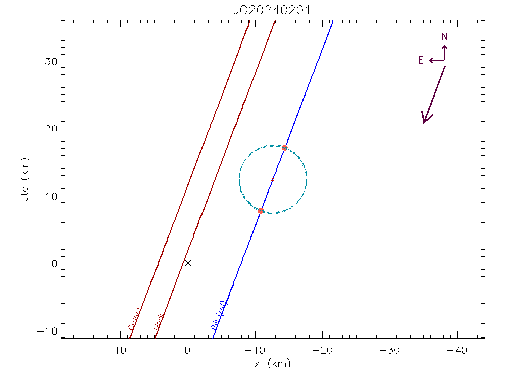
The three diagonal lines show the apparent path of the star relative to the object during the occultation. Red lines are for measurements that did not see the star disappear for this object. The blue line is for a positive detection, and the orange dots show when the star first disappeared and then reappeared. All of my occultation plots use the same color scheme. There is an ‘X’ on the plot to show where the JPL orbit predicted the position of the asteroid would be. Since this is a binary asteroid, that prediction is for the center of mass. The circle is forced to a diameter of 10 km according to Simpson’s report. The position adjusts to agree with the orange dots. Given the assumption of a circular shape, this fit shows the smallest size that is consistent with the occultation data. The area of this circle is 79 km2.
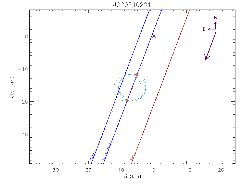
The same exercise is repeated for the satellite. In the plot above, the diameter is forced to 8.3 km as given in the report. The Graem chord is shown as blue for a positive, but the timing data is plotted with an open circle. This indicates that the data are not used for the fit, though it is useful to see it. The dashed circles show a crude attempt at indicating the uncertainty of the circle fit. The ‘X’ on this plot is in the same absolute place in the sky as for the other plot. The area of this circle is 54 km2.
Here we run into the first conflict. The total area from these two diameters is 133 km2, larger than the total area from other constraints. The upper limit on the other constraint is 125 km, and that’s pretty close to being in range, but formally the occultation result is too high. Quite frankly, I see this level of inconsistency between occultations and measurements from systems like NEOWISE and AKARI and I normally wouldn’t worry too much about this conflict. It is worrying that the occultation result is really just a lower bound, and anything bigger makes the discrepancy worse. I really don’t like answers that lie at the edge of the measurements. Here we have a result that pushed both data sets to their edge.
The second conflict is more worrisome. Recall that the Gaia data suggests the brightness ratio is f = 0.3 ± 0.13. The area ratio gives a value of 0.68. That is nearly 3σ away from the Gaia constraint. If the uncertainty is correct, there is only a 2% chance that the measurement is good. Here we have three independent constraints, and none of them are consistent.
Discrepancies like this are common in scientific research. The easiest way to resolve it is to make additional measurements as well as devise new experiments to get at the truth of the situation. However, we are now trying to make a new measurement, and the deployment plan for the upcoming occultation provides a chance to solve the problem. At this point, the important question to address is whether these discrepancies will affect the outcome of the campaign.
Resolving the conflict
My preferred approach is to examine the assumptions underlying the interpretation to see if those assumptions can be altered enough to reconcile the conflict. There may be multiple scenarios that will work. Alternatively, there may be no way to explain the data. No matter what, it’s essential to take what we learn from this exercise to consider how to adapt the deployment plan to get the answers we seek. I also want to optimize the observational effort to get as much data as we can. From here on, everything comes down to a judgment call. It is also critical to avoid emotions like loyalty to a technique or dataset to stand in the way of success. Question everything.
Let’s question the diameters from the occultation analysis first. What does it take to get a good match with the Gaia brightness ratio (f) constraint? In the following, I’m going to use the subscript 0 to refer to the larger body (primary), and 1 stands for the satellite (secondary). Sticking with the assumption of circles gives us only one option. D1 is already as small as it can be. Making it larger only makes f larger. We can match the brightness ratio if D0 = 15.1 km. The plot below shows what happens when this diameter is fit to the data.
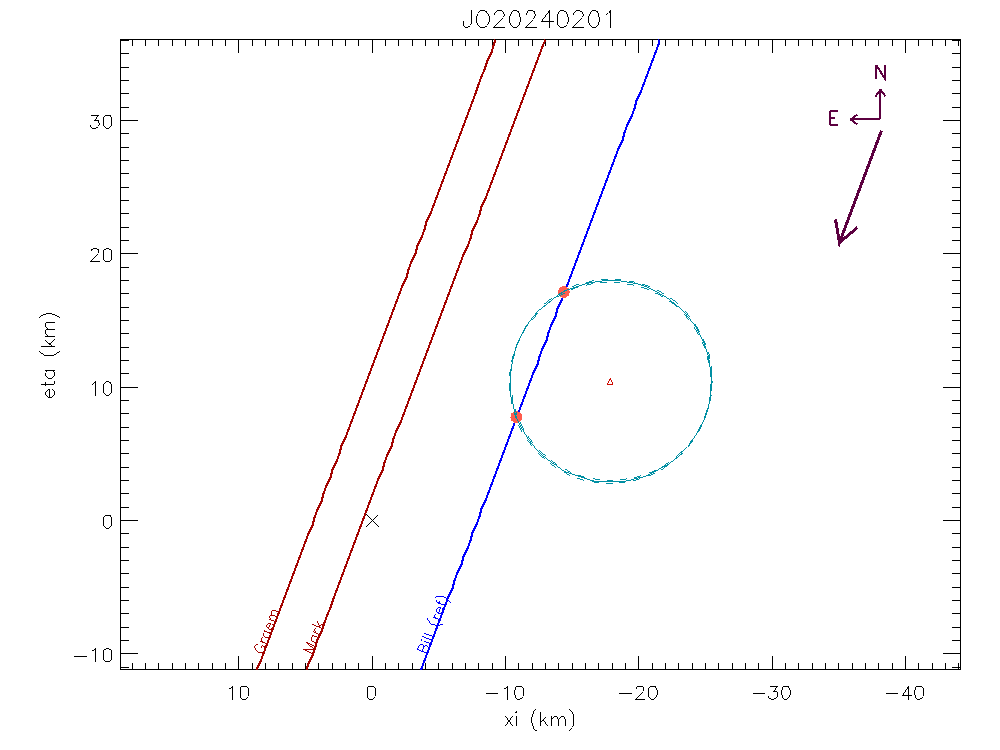
Note that the circle can’t be on the left side of the line. This is excluded because of the other datasets. But, here you see that there is no problem at all with the larger diameter, at least for the occultation data. Unfortunately, the total area becomes 233 km,2 and that is nearly double what we expect from other data. This option really doesn’t work. In fact, I cannot find a resolution to the conflict given the assumption of circular profiles. Sticking with circles requires dropping one of the three constraints.
There is no getting around that a circular profile for the satellite starts us off with too much area if we want to keep the Gaia constraint. If we consider an elliptical profile, the area will go down. With an ellipse, we also have to worry about its orientation. For a binary asteroid like this, the long axis should be aligned with the other body, and I’ve forced that to be so. Dropping the axis ratio to 0.7 requires scaling up the long axis to 9 km, and this brings the area down to 45 km2. That isn’t much of a change, and this is the best I can do with this approach. The area allowed for the main body drops to 150 km,2 but that is still too big.
What if we adjust the flux ratio? It’s easy to justify 1σ, making f = 0.45. Keeping the lower elliptical area of the satellite, this gets the area of the primary allowed down to 100 km2, closer but still too big. How about 2σ? This is less likely but not impossible, and it gets the primary area down to 80 km2 for a total of 125 km2. Let’s share the pain of the area and the f constraint and go for f = 0.52 (1.7σ off). The total area is now 132 km2.
We could make this adjustment on the primary as well. Let’s keep f = 0.52 and the slightly elliptical satellite to make things a little easier. At this point I’m really trying to get a very different and somewhat extreme option. I can match the area constraint with the larger f using a 15×7.5 km ellipse for the primary. The angle of the ellipse matches the secondary. I’m drawing inspiration from the Jupiter Trojan asteroid Polymele, which has very similar properties. The next two plots show this case.
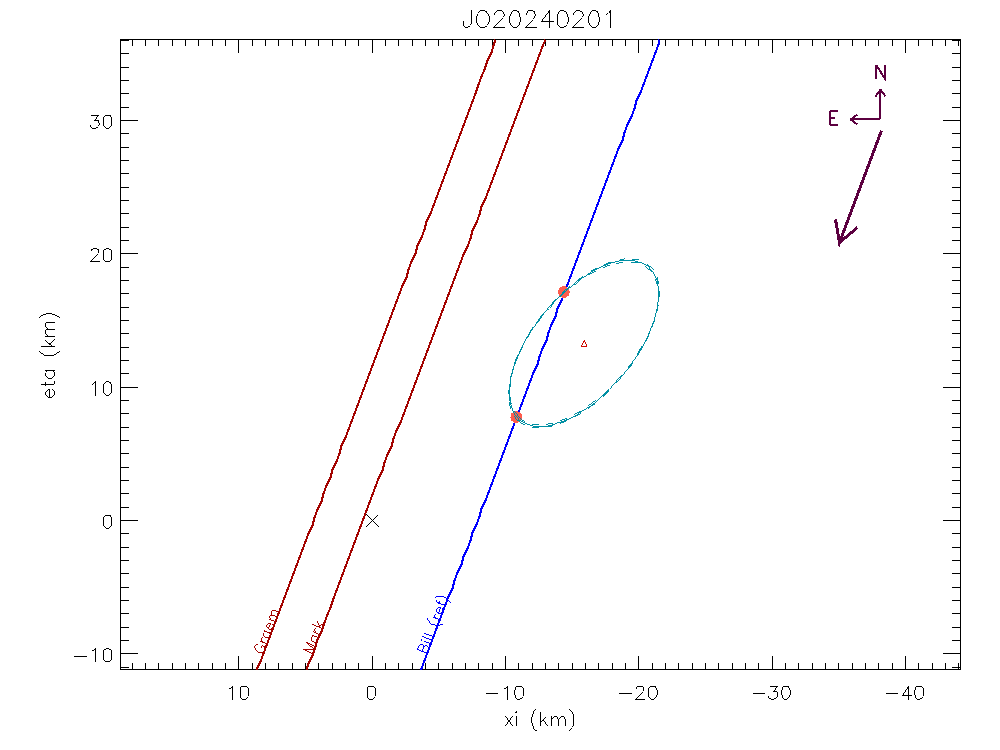
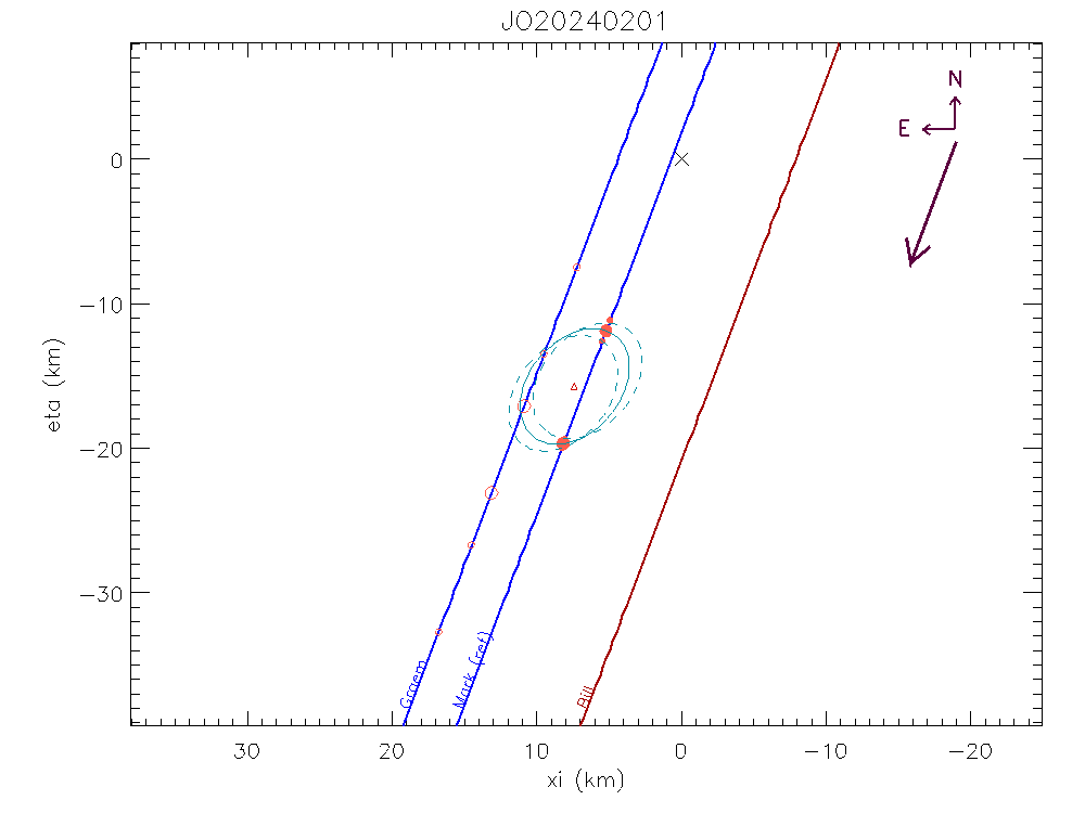
This gives us two cases to take to the prediction for the upcoming occultation. Case 1: circular, D0 = 10 km, D1 = 8.3 km. Case 2: primary 15×7.5 km and secondary 9×6.3 km.
Prediction for 2026-07-21
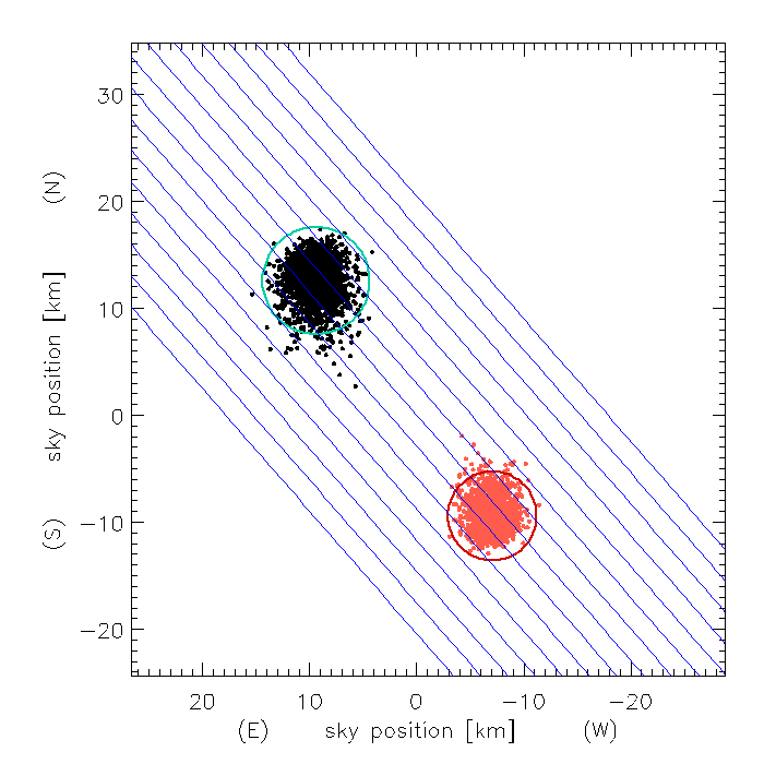
Similar to the previous post, I need to start with where the body centers are to get the bounds of the region to cover. In this case, I need to define the mass ratio, and for that I need three axes. Case 1 becomes 10×10×10 km for the primary and 8.3×8.3×8.3 km for the secondary. The mass ratio in this case is 0.57. Remember that this case is inconsistent with the Gaia constraint but works for the other two. The sky plane position clouds for this case are shown below. In this case, the predicted centerline varies between ±6.3 km. The circles are drawn at the average position of the clouds.
I have defined Case 2 as 15x15x7.5 km for the primary and 9.0x6.3x6.3 km for the secondary. The mass ratio here is 0.21, and this case is moderately consistent with all constraints. The sharp-eyed among you may notice an interesting difference between the two objects. The primary, as I’ve defined it here, is a highly oblate spheroid, similar in its shape to Polymele. The secondary is a prolate spheroid, similarly to Polymele’s satellite.
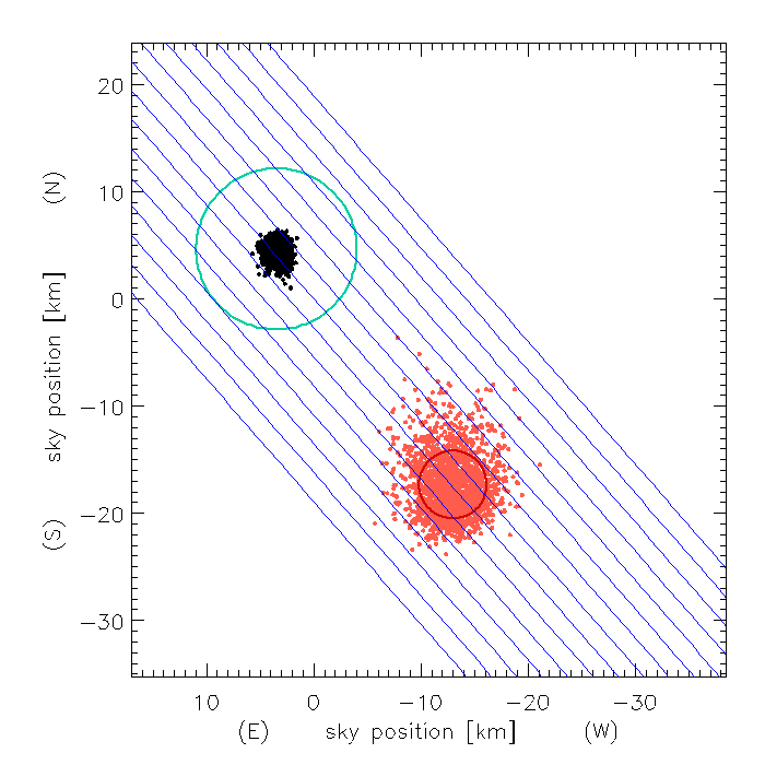
In both of these cases, I have superimposed a set of observing tracks. These are not yet the final tracks but illustrate one option. Here I have a pattern for 15 telescopes spread over the range where the two objects could be. Case 2 has a broader pattern for the satellite, and this is the one that sets the range of sky I want to cover. I have used circles in Case 2 instead of the ellipses I expect; it’s simpler that way. The diameter I picked is the intermediate axis of the spheroid dimensions. I’m guessing here, but I imagine how the orbit looks and how the objects would be oriented with respect to each other. For the observing pattern, all we really care about is the size perpendicular to the shadow motion, and the circles are good enough to show that.
The spacing between tracks is 1.78 km. For case 1, we could expect 4-5 chords on the primary and 4 chords on the secondary. For case 2, we would get 8-9 chords on the primary and 3-4 chords on the secondary. In either case, that would be a very nice result.
I have added some extra stations beyond where this analysis indicates the objects could be. The point cloud shows the uncertainties in the mutual orbit, but these are only the formal random errors. I think there could be systematic errors in the orbit fit that are not included here. Those errors would cause the angle between the two bodies to be different and would drag these point clouds along with it. What I have drawn is a wild guess, and I may yet modify this before the final deployment decision. I’m hoping to learn more about the choices the Paris group made in their orbit fit.
The good news with this revised plan is that we can expect to get better limb profiles with fewer stations than in the old (incorrect) plan. The main reasons for this are that in covering the satellite position, we automatically get the primary and don’t need extra stations for that. Moreover, the expected size of the satellite is bigger, and we can afford a slightly larger spacing, further reducing the number of stations required.
I have one final worry. I have been comparing the 2024 occultation against the area constraint from NEOWISE and AKARI. For ellipsoidal shapes, the projected area changes as they rotate. I can only assume the other data provide an average, but it is possible that the 2024 occultation records something closer to the maximum area. If so, the discrepancies are even larger than what I’ve described here. I don’t see a way out of this conundrum, so we’ll just have to adjust the deployment to be more conservative.